Next: 3. System Description Up: Fast Transformation-Based Learning Toolkit Previous: 1. Preface Contents

Subsections

2. An Introduction to Transformation-Based Learning

In 1992, Eric Brill introduced the formalism of the transformation-based learning algorithm in its current formulation, but probably a more well-known reference to the technique is Eric Brill's article from 1995, [Bri95].

The central idea behind transformation based learning (henceforth TBL) is to start with some simple solution to the problem, and apply transformations - at each step the transformation which results in the largest benefit is selected and applied to the problem. The algorithm stops when the selected transformation does not modify the data in enough places, or there are no more transformations to be selected.

While TBL can be used in a more general setup, the toolkit we are describing here is merely concerned with classification tasks, where the goal is to assign classifications to a set of samples. Although this assumption might be restrictive (not all tasks of interest may be transformed into a classification task - e.g. parsing), most natural language related tasks can be cast as classification tasks. It is not inconceivable, though, that an extension of the current toolkit for such tasks might be build, but some extensive modifications to the code are needed.

The fast TBL system (henceforth fnTBL^2.1) implements ideas from 3 articles: [FHN00], [NF01] and [FN01]. However, for the time being, the probability generation is buggy and it should not be used. As soon as we will find time, we will re-integrate the module back into the code.

2.1 The Algorithm Description

To make the presentation clearer, we will introduce some notations that will be used throughout the documentation (the notation is compatible with the above-mentioned articles):

X will denote the space of samples. How a sample is represented is dependent on the task. For example, in prepositional phrase attachment (the problem of deciding the point of attachment of a prepositional phrase), a sample can be formed from a sentence by extracting the head verb of the main verb phrase, the head noun of the noun, the preposition and the head noun of the noun phrase following the preposition:

$\displaystyle \textrm{I washed the shirt with the pockets}\, \Rightarrow \, \left( \textrm{washed},\textrm{shirt},\textrm{with},\textrm{pocket}\right)$

In part-of-speech tagging (the task of assigning a label to each word in a sentence, corresponding to its part-of-speech function), a sample might be represented as the word itself

$\displaystyle \textrm{the}_{\textrm{DT}}\textrm{ car}_{\textrm{NN}}\textrm{ }\l... ...{\textrm{DT}}\textrm{ road}_{\textrm{NN}}\textrm{ }\Rightarrow \textrm{ exited}$

This example is contrasting with the previous one in the following way: in the first one the samples in the training set form a set (the samples are independent), while in the second one they form a sequence (they are interdependent). TBL (and fnTBL in particular) can handle easily both cases; in fact, in the case when they are interdependent, the TBL shows it's full learning power. In the case where the samples are independent, it might be wise to try also some other method (decision trees, for instance), as the greedy approach of TBL can sometimes lead to sub-optimal results. Still, TBL possesses an advantage over standard machine learning techniques such as decision trees and decision lists, as it's error driven, therefore optimizing directly the error-rate (rather than other presumably correlated metrics, such as entropy or Gini index).
$\mathcal{C}$ will denote the set of possible classifications of the samples. For example, in the first task presented at point 1. the classification set $\mathcal{C}$ consists of the valid POS tags (NN, NNS, VBP, etc), while in the second case the set $\mathcal{C}$ consists of the labels s and n, corresponding to the verb attachment and noun attachment, respectively.
$\mathcal{S}$ will denote the state space $\mathcal{X}\times \mathcal{C}$ (the cross-product between the sample space and the classification space - each point in this space will be a pair of a sample and a classification)
$\pi$ will usually denote a predicate defined on the space $\mathcal{S}^{+}$ - basically a predicate on a sequence of states. For instance, in the part-of-speech case, $\pi$ might be

$\displaystyle \color{blue}\left( \textrm{word}_{-1},\textrm{tag}_{-1}\right) =\... ...{word}_{0},\textrm{tag}_{0}\right) =\left( \textrm{exited},\textrm{VBD}\right)$

or

$\displaystyle \textrm{word}_{-1}=\textrm{the}$
A rule r is defined as a pair ( $\pi$ ,) of a predicate and a target state, and it will be written as $\pi$ $\Rightarrow$ c for simplicity. A rule r=( $\pi$ ,) is said to apply on a sample if the predicate $\pi$ returns true on the sample . Examples of rules include

$\displaystyle \textrm{preposition}=\textrm{of }\Rightarrow \textrm{ attachment}\leftarrow \textrm{n}$

and

$\displaystyle \color{blue}\textrm{pos}_{-1}=\textrm{MD }\color{red}\textrm{and}... ...{VBD }\color{black}\Rightarrow \color{blue}\textrm{ pos}\leftarrow \textrm{VBN}$

Obviously, if the samples are interdependent, then the application of a rule will be context-dependent.
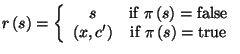
Given a state $s=\left( x,c\right)$ and a rule $r=\left( \pi ,c'\right)$ , the state resulting from applying rule to state , $r\left( s\right)$ , is defined as

$\displaystyle r\left( s\right) =\left\{ \begin{array}{cc} s & \textrm{if }\pi \... ...,c'\right) & \textrm{if }\pi \left( s\right) =\textrm{true} \end{array}\right.$
We assume that we have some labeled training data which can be either a set of samples, or a sequence of samples, depending on whether the samples are interdependent or not; We also assume the existence of some test data $\overline{T}$ on which to compute performance evaluations.
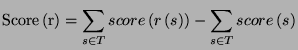
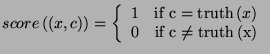
The score associated with a rule $r=\left( \pi ,c\right)$ is usually the difference in performance (on the training data) that results from applying the rule:

$\displaystyle \textrm{Score}\left( \textrm{r}\right) =\sum _{s\in T}score\left( r\left( s\right) \right) -\sum _{s\in T}score\left( s\right)$

where

$\displaystyle score\left( \left( x,c\right) \right) =\left\{ \begin{array}{cc} ... ...& \textrm{if c}\neq \textrm{truth}\left( \textrm{x}\right) \end{array}\right.$

The TBL algorithm can be now described as follows:

Initialize each sample in the training data with a classification (e.g. for each sample determine its most likely classification ); let $T_{0}$ be the starting training data.
Considering all the transformations (rules) to the training data $T_{k}$ , select the one with the highest score

$\displaystyle \textrm{Score}\left( \textrm{r}\right)$

and apply it to the training data to obtain

$\displaystyle T_{k+1}=r\left( T_{k}\right) =\left\{ r\left( s\right) \vert s\in T_{k}\right\}$

If there are no more possible transformations, or $\textrm{Score}\left( \textrm{r}\right) \leq \theta$ , stop^2.2.
$k\leftarrow k+1$
Repeat from step 2.

An easy observation that needs to be made is that the pseudo-code presented above is an algorithm, i.e. it will finish on any data that is given. The argument is simple: let us denote the number of errors in $T_{k}$ by $e_{k}$ . Then we have the following recurrence:

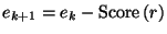$\displaystyle e_{k+1}=e_{k}-\textrm{Score}\left( r\right)$

(2.1)

Since

$\displaystyle \textrm{Score}\left( \textrm{r}\right) >\theta \geq 0$

at each stage where we apply a rule, (2.1) implies that $e_{k+1}<e_{k}$ for any

. Since $e_{k}\in \mathbbm {N}$ , it results that the algorithm will stop at some point in time, therefore avoiding, for instance, garden paths.

2.2 The Speedup

The most expensive step in the TBL computation is the computation of the rules' score. There have been many approaches that try to solve the problem in different ways:

In Brill's tagger [Bri95] (probably the most used TBL software package), the rules are regenerated at each step: only the rules that correct the errors are generated and the good counts are computed this way; then they are examined in the decreasing order of their good counts and the bad counts are computed by applying the rules to each sample -- this approach has the advantage that it can stop early (i.e. not evaluate rules whose score cannot be better than the best rule found so far). The disadvantage is that it slows down considerably as the best rule score decreases.
Ramshaw & Marcus [RM94] proposed a different approach: for each rule store all the positions in the corpus where it applies and for each sample store the list of rules that apply to it. This trick makes the update very fast, but unfortunately requires very large amounts of memory.
Samuel [Sam98] presented a Monte-Carlo approach to TBL, where only a part of the rule space is explored to determine the ``best'' transformation to apply to the data.
Lager, in his $\mu$ TBL system [Lag99], implements an efficient Prolog version of TBL, which achieves speed-ups by ``lazy'' learning.

fnTBL (as described in [NF01], provided with the distribution) achieves its speedup by generating the rules both for the good and bad counts computation. The main idea is to store the rule counts and to recompute them as necessary, when a newly selected rule gets applied to the corpus. The advantage is that only samples in the vicinity of the application of the best rule need to be examined and the rules that apply on them need to have their counts updated -- and to identify those rules, we are ``generating'' them -- using the set of templates to identify the rules that apply on those positions and update their counts (good and bad) if necessary. This approach can obtain up to 2 orders of magnitude speed-up relative to the approach present in Brill's tagger.

Next: 3. System Description Up: Fast Transformation-Based Learning Toolkit Previous: 1. Preface Contents

Radu Florian 2001-09-12